Intestinal Organoid

This tutorial uses the intestine organoid data from Battich, et al (2020). Based on the original paper, the differentiation process happens from stem cells to two distinct branches, secretory and enterocyte.

In this tutorial, we will walk you through the workflow of UniTVelo analysis and utilizing regression \(R^2\) to identify genes contributes to branching.

Intestine organoid dataset has been used in other velocity calculation methods with the help of metabolic labelling data. Here with UniTVelo, only transcriptomics data are used as input.

[1]:

import scvelo as scv
scv.settings.verbosity = 0
import unitvelo as utv

(Running UniTVelo 0.1.0)
2022-03-31 14:22:17

[7]:

dataset = '../data/Organoids/organoids.h5ad'
label = 'cell_type'
exp_metrics = {}

[8]:

adata = scv.read(dataset)
adata

[8]:

AnnData object with n_obs × n_vars = 3831 × 9157
    obs: 'well_id', 'batch_id', 'treatment_id', 'log10_gfp', 'som_cluster_id', 'monocle_branch_id', 'monocle_pseudotime', 'rotated_umap1', 'rotated_umap2', 'cell_type'
    var: 'gene'
    obsm: 'X_umap'
    layers: 'spliced', 'unspliced'

[9]:

cluster_edges = [
    ("Stem cells", "TA cells"),
    ("Stem cells", "Goblet cells")]

[10]:

adata = scv.read(dataset)
cell_mapper = {
    '1': 'Enterocytes',
    '2': 'Enterocytes',
    '3': 'Enteroendocrine',
    '4': 'Enteroendocrine progenitor',
    '5': 'Tuft cells',
    '6': 'TA cells',
    '7': 'TA cells',
    '8': 'Stem cells',
    '9': 'Paneth cells',
    '10': 'Goblet cells',
    '11': 'Stem cells',
}
adata.obs['cell_type'] = adata.obs.som_cluster_id.map(cell_mapper).astype('str')
adata.write(dataset, compression='gzip')

scVelo stochastic

[5]:

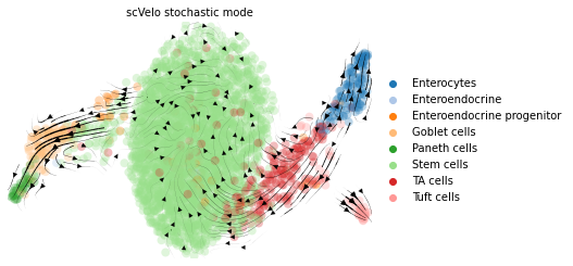
title = 'scVelo stochastic mode'
adata.uns['datapath'] = dataset
scv.pp.filter_and_normalize(adata, min_shared_counts=20, n_top_genes=2000)
scv.pp.moments(adata, n_pcs=30, n_neighbors=30)

scv.tl.velocity(adata, mode='stochastic')

scv.tl.velocity_graph(adata)
adata.uns['cell_type_colors'] = ['#1f77b4', '#aec7e8', '#ff7f0e', '#ffbb78', '#2ca02c', '#98df8a', '#d62728', '#ff9896']
scv.pl.velocity_embedding_stream(adata, color=label, title=title, legend_loc='far right')

_images/Figure4_IntestinalOrganoid_10_1.png

[5]:

scv.pp.neighbors(adata)
adata_velo = adata[:, adata.var.loc[adata.var['velocity_genes'] == True].index]
exp_metrics["model_dyn"] = utv.evaluate(adata_velo, cluster_edges, label, 'velocity')

# Cross-Boundary Direction Correctness (A->B)
{('Stem cells', 'TA cells'): -0.09643490177153952, ('Stem cells', 'Goblet cells'): 0.19285331884716267}
Total Mean: 0.048209208537811576
# In-cluster Coherence
{'Enterocytes': 0.8242295, 'Enteroendocrine': 0.9842765, 'Enteroendocrine progenitor': 0.87248236, 'Goblet cells': 0.8201039, 'Paneth cells': 0.839217, 'Stem cells': 0.7775167, 'TA cells': 0.8600152, 'Tuft cells': 0.9146982}
Total Mean: 0.8615673780441284

scVelo dynamic

[6]:

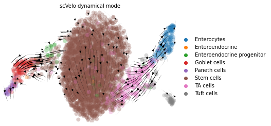
title = 'scVelo dynamical mode'
adata.uns['datapath'] = dataset
scv.pp.filter_and_normalize(adata, min_shared_counts=20, n_top_genes=2000)
scv.pp.moments(adata, n_pcs=30, n_neighbors=30)

scv.tl.recover_dynamics(adata, n_jobs=20)
scv.tl.velocity(adata, mode='dynamical')

scv.tl.velocity_graph(adata)
scv.pl.velocity_embedding_stream(adata, color=label, title=title, legend_loc='far right')

_images/Figure4_IntestinalOrganoid_13_2.png

[7]:

scv.pp.neighbors(adata)
adata_velo = adata[:, adata.var.loc[adata.var['velocity_genes'] == True].index]
exp_metrics["model_dyn"] = utv.evaluate(adata_velo, cluster_edges, label, 'velocity')

# Cross-Boundary Direction Correctness (A->B)
{('Stem cells', 'TA cells'): -0.05054847599892724, ('Stem cells', 'Goblet cells'): 0.1815118434010139}
Total Mean: 0.06548168370104332
# In-cluster Coherence
{'Enterocytes': 0.7199606522659602, 'Enteroendocrine': 0.9669398810968225, 'Enteroendocrine progenitor': 0.843149997812989, 'Goblet cells': 0.6769492431605317, 'Paneth cells': 0.6947521817913263, 'Stem cells': 0.7846342928623831, 'TA cells': 0.8228564298220513, 'Tuft cells': 0.9238745465967951}
Total Mean: 0.8041396531761074

[7]:

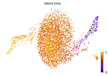
scv.tl.latent_time(adata)
scv.pl.scatter(adata, color='latent_time', color_map='gnuplot', size=20)

_images/Figure4_IntestinalOrganoid_15_0.png

UniTVelo

UniTVelo requires a configuration file as input. You may sub-class it from base config file config.py and override the parameters you need to change (demonstrated below). For the details and comments of each parameter, please refer to config.py.

Specifically, IROOT represents how cells time should be initialized, default None (based on the exact order of input expression matrix).
We also provide two other initialization options, 1) Gulati, et al (2020) has demonstated that gene counts are highly correlated with developmental status 2) diffustion pseudotime based initialization
Since gene-specific time is unified and the phase portraits of some genes are monotonically changed, wrong initialization might result in local optimum with reversed directionality.
If velo_config.IROOT = None works unsatisfactorily, we recommend change IROOT parameter or alternatively, set velo_config.NUM_REP = 2 to enabel multiple initializations.

[8]:

velo_config = utv.config.Configuration()
velo_config.R2_ADJUST = True
velo_config.IROOT = 'Stem cells'
velo_config.FIT_OPTION = '1'

[10]:

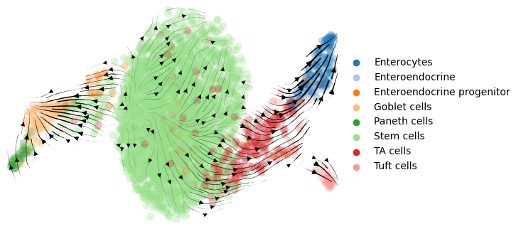
adata = utv.run_model(dataset, label, config_file=velo_config)
adata.uns['cell_type_colors'] = ['#1f77b4', '#aec7e8', '#ff7f0e', '#ffbb78', '#2ca02c', '#98df8a', '#d62728', '#ff9896']
scv.pl.velocity_embedding_stream(adata, color=adata.uns['label'], dpi=100, title='',
    legend_loc='far right')

-------> Model Configuration Settings <-------

 GPU: 2 FIG_DIR: ./figures/     BASE_FUNCTION: Gaussian
 GENERAL: Curve BASIS: None     N_TOP_GENES: 2000
 OFFSET_GENES: False    FILTER_CELLS: False     EXAMINE_GENE: False
 RESCALE_TIME: False    RESCALE_DATA: True      R2_ADJUST: True
 IROOT: Stem cells      NUM_REPEAT: 1   FIT_OPTION: 1
 DENSITY: SVD   REORDER_CELL: Soft_Reorder      AGGREGATE_T: True
 ASSIGN_POS_U: False    WIN_SIZE: 50    LEARNING_RATE: 0.01
 MAX_ITER: 10000        USE_RAW: False  RAW_GENES: False

---> # of velocity genes used 433
---> # of velocity genes used 414
---> # of velocity genes used 414
---> Use Diffusion Pseudotime as initial.

_images/Figure4_IntestinalOrganoid_20_2.png

_images/Figure4_IntestinalOrganoid_20_4.png

[6]:

scv.pp.neighbors(adata)
adata_velo = adata[:, adata.var.loc[adata.var['velocity_genes'] == True].index]
exp_metrics["model_dyn"] = utv.evaluate(adata_velo, cluster_edges, label, 'velocity')

# Cross-Boundary Direction Correctness (A->B)
{('Stem cells', 'TA cells'): 0.31262964284932904, ('Stem cells', 'Goblet cells'): 0.8771414068365261}
Total Mean: 0.5948855248429276
# In-cluster Coherence
{'Enterocytes': 0.9587416014203398, 'Enteroendocrine': 0.996026293460715, 'Enteroendocrine progenitor': 0.9934198592433778, 'Goblet cells': 0.9895047323373496, 'Paneth cells': 0.9921224640938455, 'Stem cells': 0.9917418236918903, 'TA cells': 0.9589615744200212, 'Tuft cells': 0.9773175395058773}
Total Mean: 0.982229486021677

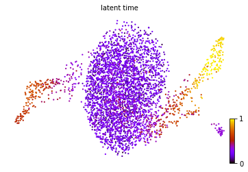
[7]:

scv.tl.latent_time(adata, min_likelihood=None)
scv.pl.scatter(adata, color='latent_time', color_map='gnuplot', size=20)

_images/Figure4_IntestinalOrganoid_22_0.png

\(R^2\) for Informative Genes

[7]:

subvar = adata.var.loc[adata.var['velocity_genes'] == True]
sub = adata[:, subvar.index]

[9]:

import seaborn as sns
import matplotlib.pyplot as plt
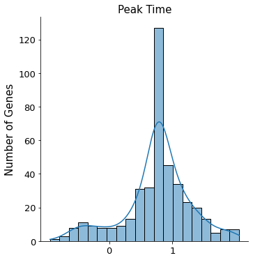
sns.displot(sub.var['fit_t0'].values, kde=True, bins=20)
plt.xticks([0, 1], fontsize=13)
plt.yticks(fontsize=13)
plt.ylabel('Number of Genes', fontsize=15)
plt.title('Peak Time', fontsize=15)

[9]:

Text(0.5, 1.0, 'Peak Time')

_images/Figure4_IntestinalOrganoid_25_1.png

[8]:

r2 = sub.var[['fit_t0', 'fit_sr2', 'fit_ur2']].sort_values(by=['fit_sr2'], ascending=False)
r2

[8]:

	fit_t0	fit_r2
index
Dgat1	0.773396	0.903234
Gsta4	0.953815	0.887514
Cyp2c66	0.763647	0.886013
Cyp2c65	0.761451	0.878404
Slc2a2	0.752518	0.873184
...	...	...
Edn1	1.871733	-0.015091
Tmem176b	0.774602	-0.017087
Gnai2	1.330305	-0.037739
Chgb	1.595687	-0.038026
Krt18	1.449424	-0.128269

414 rows × 2 columns

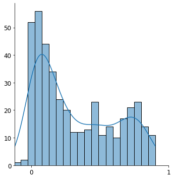
[14]:

sns.displot(r2['fit_sr2'].values, kde=True, bins=20)
plt.xlim([-0.12, 0.89])
plt.xticks([0, 1], fontsize=12)
plt.yticks(fontsize=12)
plt.xlabel('')
plt.ylabel('')

[14]:

Text(10.049999999999997, 0.5, '')

_images/Figure4_IntestinalOrganoid_27_1.png

[12]:

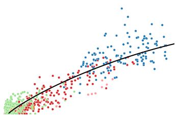
utv.pl.plot_range('Gsta4', adata, velo_config, show_legend=False, show_ax=False)

_images/Figure4_IntestinalOrganoid_28_0.png

[13]:

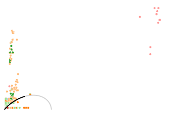
utv.pl.plot_range('Atp2a3', adata, velo_config, show_legend=False, show_ax=False)

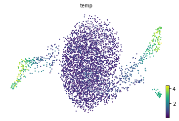
_images/Figure4_IntestinalOrganoid_29_0.png

[11]:

gene_name = 'Muc13'
adata.obs['temp'] = adata[:, gene_name].layers['Ms']
scv.pl.scatter(adata, color='temp', color_map='viridis', size=20)

_images/Figure4_IntestinalOrganoid_30_0.png

Detailed clusters

[ ]:

cell_mapper = {
    '1': 'Enterocytes',
    '2': 'Enterocytes',
    '3': 'Enteroendocrine',
    '4': 'Enteroendocrine progenitor',
    '5': 'Tuft cells',
    '6': 'TA cells',
    '7': 'TA cells',
    '8': 'Stem cells',
    '9': 'Paneth cells',
    '10': 'Goblet cells',
    '11': 'Stem cells',
}
adata.obs['cell_type'] = adata.obs.som_cluster_id.map(cell_mapper).astype('str')

[ ]:

scv.pl.velocity_embedding_stream(adata, color='cell_type', dpi=300, legend_loc='far right', title='', save='Organoids_Generalized Option 1_Detailed.png')

[ ]:

cluster_edges = [
    ("Stem cells", "Goblet cells"),
    ("Stem cells", "TA cells"),
    ("Enteroendocrine progenitor", "Goblet cells")]