Human BoneMarrow
Human bonemarrow dataset used in this tutorial is acquired from Setty et al. (2019). Bone marrow plays an crucial role in new blood cell production and contributes the generation of certain immune cells.
This dataset can be used to detect essential parts of hematopoietic differentiation and possibly the key transcription factors that contributes to the fate choice of cells within lineage.
As annotated in original paper, this dataset has three terminal states starting from HSCs, 1) erythroids, 2) monocytes and dendritic cells (DC) and 3) common lymphoid progenitor cells (CLP).
[1]:
import scvelo as scv
scv.settings.verbosity = 0
import unitvelo as utv
(Running UniTVelo 0.1.0)
2022-03-31 16:41:28
[2]:
adata = scv.datasets.bonemarrow()
adata
[2]:
AnnData object with n_obs × n_vars = 5780 × 14319
    obs: 'clusters', 'palantir_pseudotime'
    uns: 'clusters_colors'
    obsm: 'X_tsne'
    layers: 'spliced', 'unspliced'
[3]:
# dataset = '../data/BoneHuman/adata.h5ad'
dataset = './data/BoneMarrow/human_cd34_bone_marrow.h5ad'
label = 'clusters'
exp_metrics = {}
Parameter cluster_edges is for algorithm evaluation purpose given expert annotated ground truth. It contains a list of tuples in which stores the source cluster and target cluster of cells.
[4]:
cluster_edges = [
    ("HSC_1", "Ery_1"),
    ("HSC_1", "HSC_2"),
    ("Ery_1", "Ery_2")]
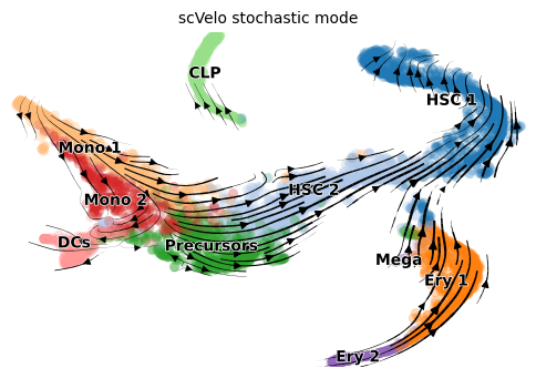
scVelo stochastic
[4]:
title = 'scVelo stochastic mode'
adata = scv.datasets.bonemarrow()
scv.pp.filter_and_normalize(adata, min_shared_counts=20, n_top_genes=2000)
scv.pp.moments(adata, n_pcs=30, n_neighbors=30)

scv.tl.velocity(adata, mode='stochastic')

scv.tl.velocity_graph(adata)
adata.uns['clusters_colors'] = ['#1f77b4', '#aec7e8', '#ff7f0e', '#ffbb78', '#2ca02c', '#98df8a', '#d62728', '#ff9896', '#9467bd', '#c5b0d5']
scv.pl.velocity_embedding_stream(adata, color=label, dpi=100, title=title)
[7]:
scv.pp.neighbors(adata)
adata_velo = adata[:, adata.var.loc[adata.var['velocity_genes'] == True].index]
exp_metrics["model_dyn"] = utv.evaluate(adata_velo, cluster_edges, label, 'velocity', 'X_tsne')
# Cross-Boundary Direction Correctness (A->B)
{('HSC_1', 'Ery_1'): -0.8610344021621074, ('HSC_1', 'HSC_2'): -0.6894453298758585, ('Ery_1', 'Ery_2'): -0.9029748019500254}
Total Mean: -0.8178181779959971
# In-cluster Coherence
{'CLP': 0.9074381, 'DCs': 0.9658171, 'Ery_1': 0.9692909, 'Ery_2': 0.9902824, 'HSC_1': 0.85452265, 'HSC_2': 0.9181577, 'Mega': 0.9639771, 'Mono_1': 0.9242185, 'Mono_2': 0.93995243, 'Precursors': 0.9324791}
Total Mean: 0.9366135597229004
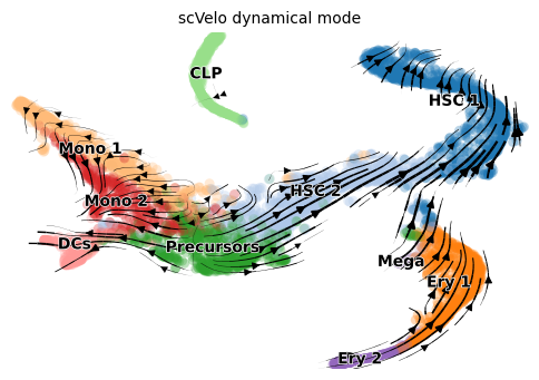
scVelo dynamic
[8]:
title = 'scVelo dynamical mode'
adata = scv.datasets.bonemarrow()
scv.pp.filter_and_normalize(adata, min_shared_counts=20, n_top_genes=2000)
scv.pp.moments(adata, n_pcs=30, n_neighbors=30)

scv.tl.recover_dynamics(adata, n_jobs=20)
scv.tl.velocity(adata, mode='dynamical')

scv.tl.velocity_graph(adata)
adata.uns['clusters_colors'] = ['#1f77b4', '#aec7e8', '#ff7f0e', '#ffbb78', '#2ca02c', '#98df8a', '#d62728', '#ff9896', '#9467bd', '#c5b0d5']
scv.pl.velocity_embedding_stream(adata, color=label, dpi=100, title=title)
[9]:
scv.pp.neighbors(adata)
adata_velo = adata[:, adata.var.loc[adata.var['velocity_genes'] == True].index]
exp_metrics["model_dyn"] = utv.evaluate(adata_velo, cluster_edges, label, 'velocity', 'X_tsne')
# Cross-Boundary Direction Correctness (A->B)
{('HSC_1', 'Ery_1'): -0.8767161904580902, ('HSC_1', 'HSC_2'): -0.7406097536917645, ('Ery_1', 'Ery_2'): -0.9011676612630122}
Total Mean: -0.8394978684709556
# In-cluster Coherence
{'CLP': 0.8011706364672638, 'DCs': 0.8831685428853896, 'Ery_1': 0.968510822837128, 'Ery_2': 0.9811672009214301, 'HSC_1': 0.93928965140427, 'HSC_2': 0.9335215285774672, 'Mega': 0.9773211685600964, 'Mono_1': 0.9071636866829598, 'Mono_2': 0.9244984234425947, 'Precursors': 0.8666819017376352}
Total Mean: 0.9182493563516235
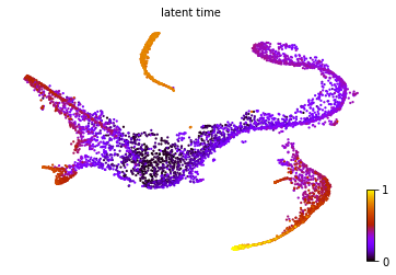
[10]:
scv.tl.latent_time(adata)
scv.pl.scatter(adata, color='latent_time', color_map='gnuplot', size=20)
UniTVelo
UniTVelo requires a configuration file as input. You may sub-class it from base config file config.py and override the parameters you need to change (demonstrated below). For the details and comments of each parameter, please refer to config.py.
[5]:
velo_config = utv.config.Configuration()
velo_config.VGENES = offset), hoping more informative genes can be included. velo_config.R2_ADJUST will be overridden under this setting.velo_config.VGENES has multiple options for selecting velocity genes as different combination of genes might affect the overall performance of the streamlines.[6]:
velo_config.VGENES = 'offset'
velo_config.R2_ADJUST = False
velo_config.IROOT = 'HSC_1'
velo_config.FIT_OPTION = '1'
[7]:
adata = utv.run_model('./data/BoneMarrow/human_cd34_bone_marrow.h5ad', label, config_file=velo_config)
adata.uns['clusters_colors'] = ['#1f77b4', '#aec7e8', '#ff7f0e', '#ffbb78', '#2ca02c', '#98df8a', '#d62728', '#ff9896', '#9467bd', '#c5b0d5']
scv.pl.velocity_embedding_stream(adata, color=adata.uns['label'], dpi=100, title='')
-------> Model Configuration Settings <-------
GPU: 2 FIG_DIR: ./figures/ BASE_FUNCTION: Gaussian
GENERAL: Curve BASIS: None N_TOP_GENES: 2000
OFFSET_GENES: True FILTER_CELLS: False EXAMINE_GENE: False
RESCALE_TIME: False RESCALE_DATA: True R2_ADJUST: False
IROOT: HSC_1 NUM_REPEAT: 1 FIT_OPTION: 1
DENSITY: SVD REORDER_CELL: Soft_Reorder AGGREGATE_T: True
ASSIGN_POS_U: False WIN_SIZE: 50 LEARNING_RATE: 0.01
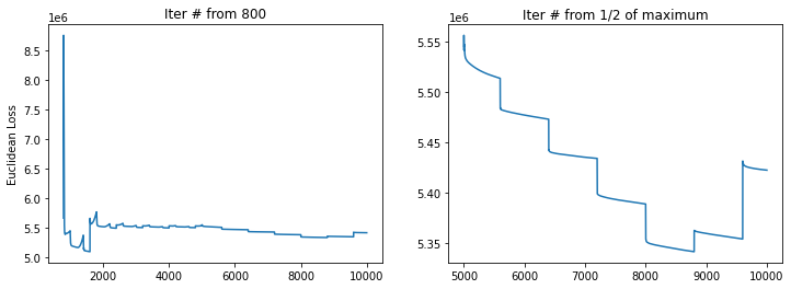
MAX_ITER: 10000 USE_RAW: False RAW_GENES: False
---> # of velocity genes used 1382
---> # of velocity genes used 1203
---> # of velocity genes used 1201
---> Use Diffusion Pseudotime as initial.
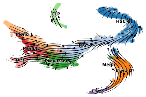
Beside visual inspections, quantitative metrics also returns a positive transition directionality (Source cluster A, Target cluster B).
[7]:
scv.pp.neighbors(adata)
adata_velo = adata[:, adata.var.loc[adata.var['velocity_genes'] == True].index]
exp_metrics["model_dyn"] = utv.evaluate(adata_velo, cluster_edges, label, 'velocity', 'X_tsne')
# Cross-Boundary Direction Correctness (A->B)
{('HSC_1', 'Ery_1'): 0.8677359570085336, ('HSC_1', 'HSC_2'): 0.7155699346392855, ('Ery_1', 'Ery_2'): 0.8316256205110811}
Total Mean: 0.8049771707196335
# In-cluster Coherence
{'CLP': 0.9722802580557224, 'DCs': 0.9804014042400353, 'Ery_1': 0.9810560277189699, 'Ery_2': 0.9851508901230266, 'HSC_1': 0.9738339141922948, 'HSC_2': 0.9756208566544446, 'Mega': 0.9861380266382976, 'Mono_1': 0.9728722765824412, 'Mono_2': 0.975874238188986, 'Precursors': 0.9715477279380238}
Total Mean: 0.9774775620332242
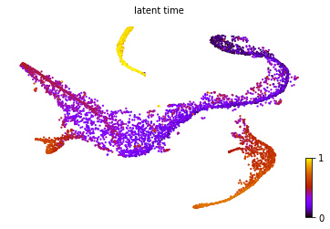
Estimated velocity along with transcriptional dynamics can be used to infer internal time of each cell, which is in accordance with Setty et al. (2019), though minor discrepancies can be observed in CLP lineage. We presume this might related to phase portraits of certain genes has high and discret expressions in CLP lineage.
[8]:
scv.tl.latent_time(adata, min_likelihood=None)
scv.pl.scatter(adata, color='latent_time', color_map='gnuplot', size=20)
Gene-level Analysis
UniTVelo automatically saves updated adata and fitted results under tempdata folder of same directory.
[9]:
adata = scv.read('./data/BoneMarrow/tempdata/temp.h5ad')
[10]:
subvar = adata.var.loc[adata.var['velocity_genes'] == True]
sub = adata[:, subvar.index]
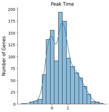
Peak time is used to roughly classify genes into three distinct catogries, - Regression gene of which it transcription profile decreases - Induction gene with the opposite behavior - Transient gene with both induced and inhibited traits combined
Since dataset is complex and the phase portraits of quite a few genes we observed does not follow the classic almond shape (termed dynamical genes by scVelo) or monotonically changes (as shown in Mouse Erythroid and Intestianl Organoid), please proceed with caution when interpreting results of which peak time is around 0.5.
[12]:
import seaborn as sns
import matplotlib.pyplot as plt
sns.displot(sub.var['fit_t0'].values, kde=True, bins=20)
plt.xticks([0, 1], fontsize=13)
plt.yticks(fontsize=13)
plt.ylabel('Number of Genes', fontsize=15)
plt.title('Peak Time', fontsize=15)
[12]:
Text(0.5, 1.0, 'Peak Time')
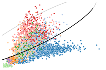
Here shows an example of repression gene, CD44. Generally the spliced counts follow a decreased manner (from upper right to lower left of the black pahse portrait), though an elevated expression can be observed in unspliced counts.
[13]:
utv.pl.plot_range('CD44', adata, velo_config,
    show_legend=False, show_ax=False)
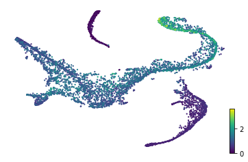
[14]:
gene_name = 'CD44'
adata.obs['temp'] = adata[:, gene_name].layers['Ms']
scv.pl.scatter(adata, color='temp', color_map='viridis', size=20, title='')
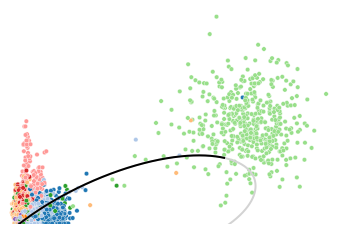
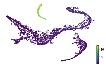
To illustrate the high but discret expressions in CLP lineage mentioned above, we use LAPTM5 as an example, which is also a poorly fitted gene.
The scatter plor of un/spliced counts shows the transcription acticity does not change much (probably decreased a little) in HSCs, erythroids and monocytes. However, a transcription burst can be observed in CLP lineage. This anomaly easily leads to erroneous or over-fitting of the phase portraits.
Though the general result can be refined with UniTVelo under unified-time setting. Fitting each gene with correct phase portrati individually still remains challenging.
[20]:
utv.pl.plot_range('LAPTM5', adata, velo_config,
    show_legend=False, show_ax=False)
[21]:
gene_name = 'LAPTM5'
adata.obs['temp'] = adata[:, gene_name].layers['Ms']
scv.pl.scatter(adata, color='temp', color_map='viridis', size=20, title='')
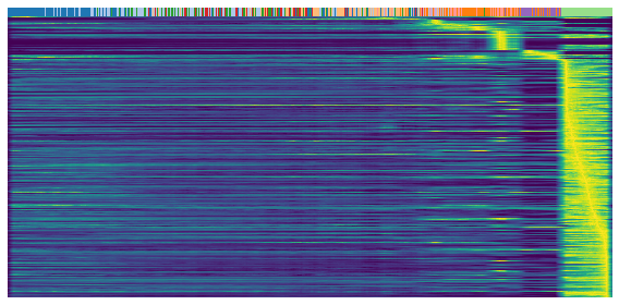
Heatmap
Heatmaps shows the expression profile (rows) againese cell ordering (columns, inferred cell time). Brighter color represents higher expression.
[16]:
adata.uns['clusters_colors'] = ['#1f77b4', '#aec7e8', '#ff7f0e', '#ffbb78', '#2ca02c', '#98df8a', '#d62728', '#ff9896', '#9467bd', '#c5b0d5']
gene = sub.var.loc[sub.var['fit_t0'] < 0.05].index # repression
scv.pl.heatmap(
    adata, var_names=gene, sortby='latent_time', yticklabels=False,
    col_color=label, n_convolve=100)
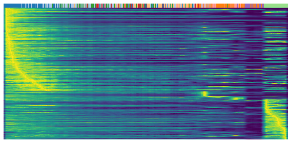
[17]:
gene = sub.var.loc[sub.var['fit_t0'] > 0.95].index # induction
scv.pl.heatmap(
    adata, var_names=gene, sortby='latent_time', yticklabels=False,
    col_color=label, n_convolve=100)